Measuring Intermittent Demand: Forecast Accuracy and Inventory Metrics

Intermittent demand where demand occurs sporadically with many periods of zero sales, presents a unique challenge for forecasters and supply chain planners. Traditional metrics for forecast accuracy can be misleading when applied to slow-moving items, and focusing solely on these can lead to suboptimal inventory decisions. This article explores which metrics to use for evaluating forecasts of intermittent demand, including accuracy measures (and their limitations) and inventory-oriented metrics. 

Understanding Intermittent Demand and Its Importance 

Intermittent demand (also called sporadic or lumpy demand) is characterized by frequent zero-demand periods and occasional spikes when orders occur. Many industries deal with intermittent demand for a significant portion of their items. For example, 

• Aerospace and defense organizations manage thousands of spare parts that rarely fail but must be available when needed; 

• Automotive aftermarket suppliers face slow-moving replacement parts; 

• Tech and IT sector handles intermittent demand for legacy components; and even 

• Specialty chemicals may sell only irregularly in niche applications. 

• Military logistics, a critical spare part might have no demand for months and then a sudden requirement (e.g., due to an equipment breakdown). 

• In retail, “long-tail” products (low-volume, niche items) also exhibit intermittent demand. 

These items often represent a large share of total stock value and are essential for service or maintenance contracts. Thus, evaluating forecast performance for intermittent demand is not just an academic exercise as it directly impacts inventory investment, service levels, and customer satisfaction. The ultimate goal is to forecast in a way that enables high product availability (to avoid costly stockouts) while controlling inventory costs for items that may sit idle for long periods. 

Why Traditional Accuracy Metrics Fall Short 

Forecast accuracy is often the first lens we apply, but standard error metrics can mislead when demand is intermittent. 

• Avoid MAPE. Despite its popularity, Mean Absolute Percentage Error is mathematically unreliable when actual demand is zero or very low which is common in intermittent demand. It produces undefined or distorted values and has long been recognized as unsuitable in both academic and practitioner circles. Worse, MAPE disproportionately penalizes low-volume series while favoring high-volume ones, skewing multi-item evaluations. 

• Use MAE or RMSE with caution. These scale-dependent metrics are more stable with zeros and frequently used in comparative evaluations. RMSE penalizes large misses more heavily, while MAE averages absolute errors. However, both can be deceptive: they are minimized by the median of the forecast, which in intermittent contexts is often zero. This means a naïve model that always forecasts zero, even when it misses actual demand, can outperform more sophisticated ones on MAE or RMSE. That’s a problem: models that appear “accurate” may be operationally useless, failing to trigger inventory replenishment when needed. 

• Monitor bias (ME or MPE). Bias remains defined even with zeros and reveals whether forecasts systematically overshoot or undershoot demand. But with intermittent series, a near-zero bias can be misleading. A few large over-forecasts might cancel out frequent under-forecasts, hiding service-level failures. Over-forecasting to improve fill rate may protect short-term operations but suggests poor model calibration in the long term. 

• Bottom line: Traditional accuracy metrics, especially those based on percentage errors, are not only mathematically unstable for intermittent demand but can actively mislead. Even well-behaved metrics like MAE or RMSE can reward forecasting models that never predict a sale. These measures may favor models that suppress inventory altogether. 

Forecast Accuracy Metrics Suited for Intermittent Demand 

To evaluate intermittent demand effectively, we need metrics that are stable with zeros, scale-independent, and aligned with decision-making. Below are several academic recommendations, along with when to use each. 

• MAAPE (Mean Arctangent Absolute Percentage Error): Proposed by Kim & Kim (2016), MAAPE uses an arctangent transformation to dampen extreme percentage errors, making it robust against outliers common in intermittent series. It behaves like MAPE for small errors but avoids distortion from rare large ones. Though not yet widely adopted in software, it’s gaining traction in research for its reliability and interpretability. 

• MdAPE (Median Absolute Percentage Error): Highlights the typical forecast error by reducing the impact of outliers. It’s useful when errors are highly skewed or dominated by a few extreme values, as is common in intermittent demand. However, it may understate risk by ignoring rare but critical large errors, so it should be used alongside other metrics that capture those extremes. 

• Probabilistic forecasts predict a range or distribution of possible outcomes instead of a single number, which is especially useful for intermittent demand where uncertainty is high. To evaluate these forecasts, use metrics like CRPS (Continuous Ranked Probability Score), which assesses the accuracy of the full predicted distribution (Wang et al. 2024). 

Inventory Metrics and Service Level Measures 

Forecast accuracy metrics provide only a partial view of forecast quality. Especially for intermittent demand, the ultimate goal is not accuracy for its own sake, but service and cost effectiveness. Therefore, it’s essential to evaluate how forecasts influence inventory and fulfillment outcomes. 

• Cycle Service Level (CSL): Indicates the proportion of replenishment cycles completed without a stockout, focusing on whether all demand was met before the next order arrived. It’s especially valuable in environments where even a single stockout is unacceptable (e.g., critical spare parts or service agreements), as it emphasizes the event of a stockout rather than the amount. 

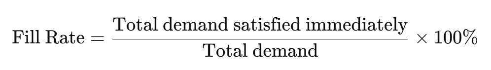
• Fill Rate (FR): Measures the percentage of total demand volume that is fulfilled immediately from available inventory, making it key in contexts where customers care about how many units they actually receive on time. Unlike CSL, fill rate captures the magnitude of stockouts and is often a better reflection of performance in high-volume or customer-facing environments. 

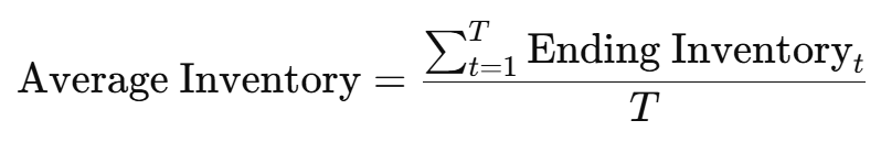
• Average Inventory: Reflects the typical amount of inventory held over time and is crucial for understanding capital investment and carrying costs. For intermittent demand, high average inventory may signal overstocking, especially if service levels don’t justify the holding cost. 

• Stockout Frequency: Tracks how often stockouts occur during defined time intervals (e.g., weekly, monthly), helping identify patterns of underperformance even if the lost demand is small. It’s especially useful for planners aiming to minimize disruption frequency rather than just the total quantity missed. 

• Backorder Level: Represents the average or cumulative amount of demand that couldn’t be fulfilled on time and remained pending. It reveals how severe the stockout impact is over time, especially in environments where demand is eventually fulfilled (e.g., B2B spare parts logistics) rather than lost. 

• Inventory Turnover: Shows how often inventory is consumed or sold relative to the stock held and serves as a general indicator of inventory efficiency. While low turnover is expected for slow-moving or strategic items, tracking it helps flag obsolete or excessive inventory across portfolios. 

• Inventory Cost (Total): Aggregates holding and stockout costs to assess the financial impact of a forecasting and replenishment strategy. It enables direct comparison of forecast performance in business terms, especially when trade-offs must be made between service and efficiency. This is the most holistic KPI when cost optimization is a priority. 

Inventory metrics should be assessed together with forecast metrics. A forecast that slightly overestimates demand may lead to better service levels by avoiding stockouts, while one with low statistical error might still underperform if it misses key demand peaks. Rankings based purely on forecast accuracy don’t always reflect real-world outcomes. The best approach is to simulate how different forecasts perform within your inventory policy and evaluate based on service levels and stock efficiency, not just model fit. 

Intermittent Forecasting in Different Industries: Examples from Academic Literature 

This section illustrates how recent research has tackled intermittent demand forecasting across sectors, highlighting practical methods that align forecasting accuracy with inventory decision-making. 

• Retail Slow-Movers (Long-tail products): A recent study by Wang et al. (2024) shows that for products with intermittent demand, forecasting methods should be evaluated not just by how statistically accurate they are, but by how well they support inventory decisions. Using real retail data, they tested a wide range of forecasting methods, including traditional Croston-based models, aggregation techniques, and machine learning. These were used to generate probabilistic forecasts, which were then combined in different ways: using equal weights, optimizing for forecast accuracy, and optimizing for inventory cost. They found that the combinations optimized for inventory cost delivered the best overall results (i.e. lower total costs and higher service levels) even when their statistical forecast scores weren’t the best. For practitioners managing long-tail inventory, this highlights the value of evaluating forecasts through the lens of inventory performance, not just statistical error. 

• Aircraft Spare Parts (Aerospace/Defense): Demand for a specific spare part (e.g., a landing gear component) might be 0 for months and then suddenly 1 or 2 when a plane is in maintenance. Here the focus is on very high service levels – stockouts could ground aircraft. Li et al. (2014) demonstrate that for aircraft spare parts with highly irregular demand, traditional forecasting methods often miss critical fluctuations, leading to overstock or stockouts. Using data from 113 A320 aircraft, they developed the MCAHR method, which decomposes demand signals into detailed components using Wavelet Packet Transform and then applies Fuzzy Neural Networks optimized with Particle Swarm Optimization to capture complex, non-linear demand patterns. This approach outperformed both traditional and advanced forecasting methods, proving especially effective for parts with erratic demand like actuator cylinders and pressure valves. For aviation supply chain professionals, this highlights the importance of using forecasting methods that can handle high variability while preserving signal detail, ensuring better stock decisions and service levels. 

• Automotive Spare Parts: Zhuang et al. (2022) show that for automotive spare parts with intermittent demand, it is critical to forecast not only how much demand will occur, but if and when it will occur. Using real aftersales data from over 3,000 SKUs, they developed a machine learning–based two-stage approach (IDCF) that first predicts demand occurrence and then predicts demand size. This approach uses LightGBM, a gradient boosting algorithm well-suited for large, complex datasets, and further improves accuracy through threshold optimization and transfer learning when historical data are limited. While it significantly reduced forecast errors (lower MASE, higher AUC), its key practical impact was reducing unnecessary replenishments while improving availability. For automotive supply chain professionals, this highlights the value of classification-driven forecasting for slow-moving parts, aligning forecasts directly with replenishment decisions to lower inventory costs while maintaining service levels. 

Across these examples, a clear principle emerges: forecast evaluation should align with business objectives, not just statistical error metrics. For critical items like aircraft parts where stockouts can halt operations, prioritizing service levels and fill rates ensures customer needs are met. For slow-moving or long-tail inventory, where excess stock ties up capital, focusing on inventory turns and holding cost reductions is key. By aligning forecasting methods and evaluation metrics with these operational priorities, supply chain teams can make forecasting a tool for smarter, goal-driven inventory management rather than a disconnected technical exercise. 

Best Practices for Evaluating Intermittent Demand Forecasts 

Use multiple metrics together to get a complete view, pairing forecast accuracy (e.g., MAAPE, Bias) with inventory metrics (e.g., fill rate, holding cost). A method with slightly higher forecast error might deliver better service levels and lower total costs depending on your priorities. 

• Know when metrics fail, as each has blind spots. For example, MAPE struggles with zero demand, and fill rate alone may hide excess inventory issues. 

• Test how accuracy improvements translate to inventory outcomes. A 15% MASE improvement may have minimal effect on service if safety stock already buffers variability, while quantile forecasting may improve availability without raising inventory. 

• Align metrics with your industry context. In high stockout-cost industries like aerospace, service levels take priority. In cost-sensitive environments, small gains in accuracy can significantly reduce holding costs. 

• Stay updated with research as methods like Croston variants, TSB, and machine learning evolve. Evaluate them not only on accuracy but also on real impacts on inventory availability and cost, ensuring forecasting improvements deliver business value.